2.4. Mass lumping#
For the use of explicit time-stepping methods in each time step the inverse of the mass matrices have to be applied. Thus it would be optimal if the basis functions are chosen such that the mass matrices are diagonal. Classical mass lumping techniques approximate the mass integrals by numerical integration rules to obtain diagonal matrices. We use a similar approach
In Section 2.3 we have defined polynomial nodal basis functions of order \(P\) with respect to nodes \(x_0,\ldots,x_P\) on the unit interval \([0,1]\) (and tensorized on the unit square/cube). Apart from the fact that we need \(x_0=0\) for the dual and \(x_P=1\) for the dual spaces we have not yet specified which nodes we choose exactly.
The main idea is now to choose the nodes such that they are the integration points of a numerical quadrature rule of as high order as possible. Since the nodal polynomials vanish in every integration node except one we expect very sparse mass matrices when using the corresponding integration rules to approximate the mass integrals.
The quadrature rules of choice are Gauss-Radau rules, where we fix, depending on whether we treat the dual or primal space, the starting or endpoint of the interval in question. As usual for Gaussian quadratures, the integration points and weights may be easily computed via a eigenvalue problem of dimension \(P+1\).
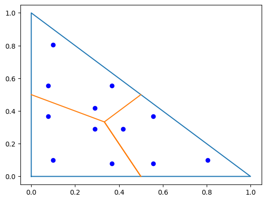
To compare the sparsity patterns of the exact mass matrices to the ones obtained by using mass lumping we have to compute the exact mass matrices. Since our basis functions are not smooth (and for the dual spaces even discontinuous) in the primal elements we may not use the standard integration rules provided by NGSolve here. The package provides dualcellspaces.GetIntegrationRules to obtain fitting quadrature formulas (Gauss rules on the reference shape transformed to the cells):
from ngsolve import *
import dualcellspaces as dcs
import matplotlib.pyplot as pl
import numpy as np

irs = dcs.GetIntegrationRules(2)
for et in irs:
  print(et)
  print(irs[et])

pl.plot([0,1,0,0],[0,0,1,0]);
pl.plot([0,1/3,0.5,1/3,0.5],[0.5,1/3,0,1/3,0.5]);

trig_points = np.array(irs[TRIG].points)
px,py = trig_points[:,0],trig_points[:,1]
pl.plot(px,py,'ob');
ET.SEGM
 locnr = -1: (0.105662, 0, 0), weight = 0.25
 locnr = -1: (0.394338, 0, 0), weight = 0.25
 locnr = -1: (0.894338, 0, 0), weight = 0.25
 locnr = -1: (0.605662, 0, 0), weight = 0.25

ET.TRIG
 locnr = -1: (0.803561, 0.0982194, 0), weight = 0.0536948
 locnr = -1: (0.555556, 0.0778847, 0), weight = 0.0416667
 locnr = -1: (0.555556, 0.36656, 0), weight = 0.0416667
 locnr = -1: (0.418661, 0.290669, 0), weight = 0.0296385
 locnr = -1: (0.0982194, 0.803561, 0), weight = 0.0536948
 locnr = -1: (0.36656, 0.555556, 0), weight = 0.0416667
 locnr = -1: (0.0778847, 0.555556, 0), weight = 0.0416667
 locnr = -1: (0.290669, 0.418661, 0), weight = 0.0296385
 locnr = -1: (0.0982194, 0.0982194, 0), weight = 0.0536948
 locnr = -1: (0.0778847, 0.36656, 0), weight = 0.0416667
 locnr = -1: (0.36656, 0.0778847, 0), weight = 0.0416667
 locnr = -1: (0.290669, 0.290669, 0), weight = 0.0296385

ET.TET
 locnr = -1: (0.725312, 0.0915628, 0.0915628), weight = 0.00999851
 locnr = -1: (0.51153, 0.0733767, 0.0733767), weight = 0.00616387
 locnr = -1: (0.51153, 0.0733767, 0.341717), weight = 0.00616387
 locnr = -1: (0.391248, 0.0610607, 0.273846), weight = 0.00365801
 locnr = -1: (0.51153, 0.341717, 0.0733767), weight = 0.00616387
 locnr = -1: (0.391248, 0.273846, 0.0610607), weight = 0.00365801
 locnr = -1: (0.391248, 0.273846, 0.273846), weight = 0.00365801
 locnr = -1: (0.316355, 0.227882, 0.227882), weight = 0.0022025
 locnr = -1: (0.0915628, 0.725312, 0.0915628), weight = 0.00999851
 locnr = -1: (0.341717, 0.51153, 0.0733767), weight = 0.00616387
 locnr = -1: (0.0733767, 0.51153, 0.0733767), weight = 0.00616387
 locnr = -1: (0.273846, 0.391248, 0.0610607), weight = 0.00365801
 locnr = -1: (0.0733767, 0.51153, 0.341717), weight = 0.00616387
 locnr = -1: (0.273846, 0.391248, 0.273846), weight = 0.00365801
 locnr = -1: (0.0610607, 0.391248, 0.273846), weight = 0.00365801
 locnr = -1: (0.227882, 0.316355, 0.227882), weight = 0.0022025
 locnr = -1: (0.0915628, 0.0915628, 0.725312), weight = 0.00999851
 locnr = -1: (0.0733767, 0.341717, 0.51153), weight = 0.00616387
 locnr = -1: (0.341717, 0.0733767, 0.51153), weight = 0.00616387
 locnr = -1: (0.273846, 0.273846, 0.391248), weight = 0.00365801
 locnr = -1: (0.0733767, 0.0733767, 0.51153), weight = 0.00616387
 locnr = -1: (0.0610607, 0.273846, 0.391248), weight = 0.00365801
 locnr = -1: (0.273846, 0.0610607, 0.391248), weight = 0.00365801
 locnr = -1: (0.227882, 0.227882, 0.316355), weight = 0.0022025
 locnr = -1: (0.0915628, 0.0915628, 0.0915628), weight = 0.00999851
 locnr = -1: (0.0733767, 0.0733767, 0.341717), weight = 0.00616387
 locnr = -1: (0.0733767, 0.341717, 0.0733767), weight = 0.00616387
 locnr = -1: (0.0610607, 0.273846, 0.273846), weight = 0.00365801
 locnr = -1: (0.341717, 0.0733767, 0.0733767), weight = 0.00616387
 locnr = -1: (0.273846, 0.0610607, 0.273846), weight = 0.00365801
 locnr = -1: (0.273846, 0.273846, 0.0610607), weight = 0.00365801
 locnr = -1: (0.227882, 0.227882, 0.227882), weight = 0.0022025
Using these IntegrationRules we may compute the exact mass matrices:
from ngsolve import *
import dualcellspaces as dcs
import matplotlib.pyplot as pl
import numpy as np
order = 3
irs = dcs.GetIntegrationRules(2*order+2)
mesh = Mesh(unit_square.GenerateMesh(maxh=0.5))
#fes = dcs.HCurlDualCells(mesh,order=order)
fes = dcs.H1PrimalCells(mesh,order=order)
u,v = fes.TnT()
M = BilinearForm(u*v*dx(intrules=irs)).Assemble().mat
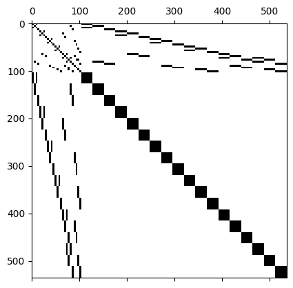
pl.spy(M.ToDense());
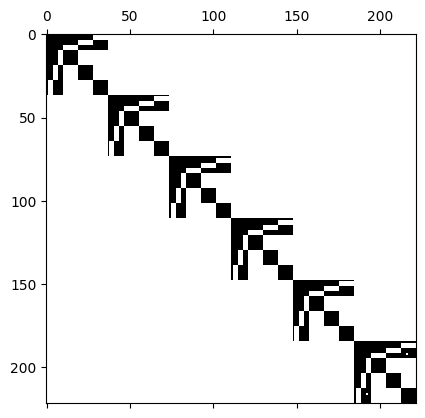
The resulting matrix can easily be seen to be block-diagonal.
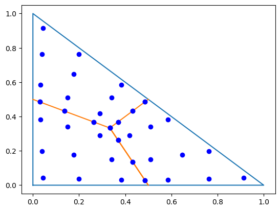
To approximate the mass matrix using the integration rule which was used in the construction of the basis functions we may obtain the IntegrationRule from the FESpace:
irs_fes = fes.GetIntegrationRules()

pl.plot([0,1,0,0],[0,0,1,0]);
pl.plot([0,1/3,0.5,1/3,0.5],[0.5,1/3,0,1/3,0.5]);

trig_points = np.array(irs_fes[TRIG].points)
px,py = trig_points[:,0],trig_points[:,1]
pl.plot(px,py,'ob');

M = BilinearForm(u*v*dx(intrules=irs_fes)).Assemble().mat
pl.figure()
pl.spy(M.ToDense());
M_diag = M.DeleteZeroElements(1e-10)
pl.figure()
pl.spy(M_diag.ToDense());

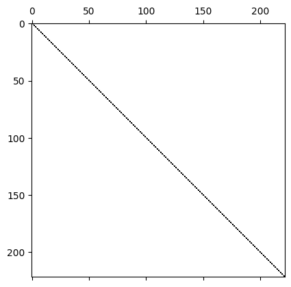
We can observe that the coupling entries between basis function of the same element are numerically zero, by construction and we obtain a diagonal matrix. For the vectorial spaces the lumped mass matrices are block diagonal:
fes_curl = dcs.HCurlDualCells(mesh,order=order)
u,v = fes_curl.TnT()

M = BilinearForm(u*v*dx(intrules=irs)).Assemble().mat
pl.spy(M.ToDense());

irs_fes_curl = fes_curl.GetIntegrationRules()
M_lumped = BilinearForm(u*v*dx(intrules=irs_fes_curl)).Assemble().mat
M_lumped = M_lumped.DeleteZeroElements(1e-10)
pl.figure()
pl.spy(M_lumped.ToDense());
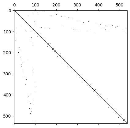
Since the entries corresponding to basis functions of the dual elements are not stored together the block structure is less obvious here.
Exploiting this block structure is implemented in the finite element spaces. The mass matrices may be accessed via FESpace.Mass:
from time import time

order = 3

irs = dcs.GetIntegrationRules(2*order+2)
mesh = Mesh(unit_cube.GenerateMesh(maxh=0.3))
fes = dcs.HCurlDualCells(mesh,order=order)

print("ndof = ",fes.ndof)

irs_fes = fes.GetIntegrationRules()
u,v = fes.TnT()

with TaskManager():
  now = time()
  M_exact = BilinearForm(u*v*dx(intrules=irs)).Assemble().mat
  exacttime = time()-now

  now = time()
  M_supersparse = fes.Mass()
  stime = time()-now

  print('#### assembling ####')
  print('exact: {}s'.format(exacttime))
  print('supersparse: {}s'.format(stime))


  now = time()
  M_exact_inv = M_exact.Inverse(inverse='sparsecholesky')
  exacttime = time()-now

  now = time()
  with TaskManager():
    M_supersparse_inv = M_supersparse.Inverse()
  stime = time()-now
  print('#### factorization ####')
  print('exact: {}s'.format(exacttime))
  print('supersparse: {}s'.format(stime))

  n = 10
  tmp = M_exact.CreateVector()
  tmp.SetRandom()
  tmp2 = M_exact.CreateVector()

  now = time()
  for i in range(n):
    tmp2.data = M_exact_inv * tmp
  exacttime = time()-now

  now = time()
  for i in range(n):
    tmp2.data = M_supersparse_inv * tmp
  stime = time()-now

  print('#### application ####')
  print('exact: {}s'.format(exacttime))
  print('supersparse: {}s'.format(stime))
ndof = 126200
#### assembling ####
exact: 7.314175367355347s
supersparse: 0.5558481216430664s
#### factorization ####
exact: 33.006203174591064s
supersparse: 0.048715829849243164s
#### application ####
exact: 1.4642248153686523s
supersparse: 0.01563549041748047s