2.2. Introduction

When solving time-domain wave-type problems using a method of lines approach one typically has the choice between implicit and explicit methods. For the former in each time-step the inverse of a system matrix composed of the mass matrix and the discrete differential operator has to be applied. Although such schemes are typically unconditionally stable (independent of the choice of the time-step) the factorization of a large matrix does not scale well for very large numbers of degrees of freedom.

For explicit methods, on the other hand in each time-step merely the inverse mass matrix has to be applied. There exist several methods to make the mass matrix as convenient for inversion as possible. The downside of explicit methods is the fact that their stability depends on the quality of the discretization, i.e., the finer the discretization, the finer is the largest admissible time-step that guarantees stability.

Reasons for explicit methods

Apart from the obvious better scaling for very large applications, explicit time-domain solvers are also interesting for frequency-domain applications:

scattering type problems

• time-domain solvers for Helmholtz (2020s e.g., [AppeloGR20])

• time-domain preconditioners (2020s, e.g., [Sto21] )

resonance type problems

• explicit eigenvalue solvers lite PINVIT, LOBPCG (early 2000s, e.g., [Kny01] )

• time-domain filters for eigenvalue problems (very recent [NW24])

State of the art

The most popular explicit methods are

Finite Difference Time Domain (FDTD) Methods

• 2e5 hits on Google scholar, 1.2e4 since 2022

• low order

• only hexahedral grids

Discontinuous Galerkin (DG) Methods

• 1.5e4 hits on Google scholar, 1.6e3 since 2022

• high order

• necessary choice of numerical fluxes, penalty parameter

While both of these methods have been around since the late 1960’s and early 1970’s FDTD is still most widely used in engineering applications.

From FDTD to the dual cell method

The main idea of the FDTD methods is the discretization of Stokes’ theorem.

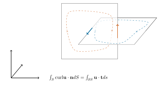
Fig. 2.1 A visualization of Stokes’ theorem.

This leads to discrete quantities on interlaced hexahedral grids.

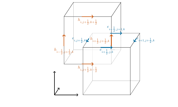
Fig. 2.2 Discrete, pointwise approximations mimmicking Stokes’ theorem.

\(h^l_{i,j,k},e^l_{i,j,k}\) are point values of the fields at points \((x_i,y_j,z_k)\) (tangential to the staggered grid) at timestep number \(l\) and satisfy

\[\begin{split}\partial_t h_{i+\tfrac{1}{2},j+\tfrac{1}{2},k}&\approx e_{i+\tfrac{1}{2},j,k}-e_{i+1,j+\tfrac{1}{2},k}-e_{i+\tfrac{1}{2},j+1,k}+e_{i,j+\tfrac{1}{2},k}\\ \partial_t e_{i+\tfrac{1}{2},j+\tfrac{1}{2},k}&\approx h_{i+\tfrac{1}{2},j+\tfrac{1}{2},k}-h_{i,j+\tfrac{1}{2},k+\tfrac{1}{2}}-h_{i-\tfrac{1}{2},j+\tfrac{1}{2},k}-h_{i,j+\tfrac{1}{2},k-\tfrac{1}{2}}\end{split}\]

The time discretization is done using a Leap-Frog time-stepping with time-step size \(\tau\),

\[\partial_t h^{l}_{i,j,k}\approx \frac{h_{i,j,k}^{l+\tfrac{1}{2}}-h_{i,j,k}^{l-\tfrac{1}{2}}}{\tau},\quad\quad\quad\partial_t e^{l+\tfrac{1}{2}}_{i,j,k}\approx \frac{e_{i,j,k}^{l+1}-e_{i,j,k}^{l}}{\tau}\]

which carries the idea of the interlaced grid to time-domain.

Goal of the dual cell method

generalize FDTD to

• high order Galerkin method

• on general (tetrahedral) grids

Basic idea of the dual cell construction

For motivation of the construction of the basis functions and spaces we start by focussing on the two dimensional problem.

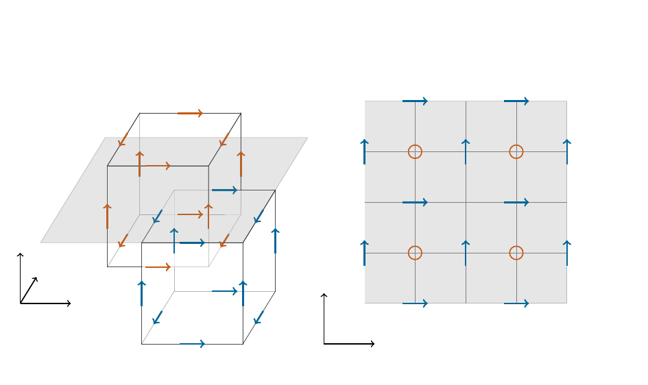
Fig. 2.3 Going to two dimensions.

Galerkin setting and high order spaces

Interpreting the scalar point values (orange circles) as piecewise constant basis functions on each element \(\mathbf C\) (dark grey, consisting of four cells) we may proceed from a finite difference setting, to a Galerkin setting.

For the vectorial unknowns the degrees of freedom are the inner tangential components between two neighbouring cells. The respective basis functions are tangentially continuous on each dual element \(\tilde {\mathbf C}\) (again consisting of four cells).

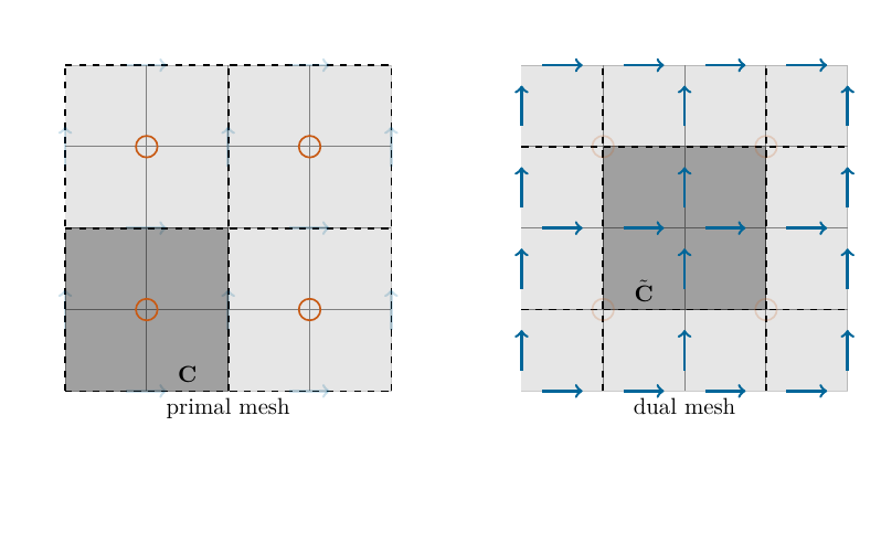
Fig. 2.4 primal and dual quad-meshes

Thus if the primal and dual elements are given by

\[\begin{split}\mathbf C_j&=\bigcup_{k=0}^3 C_{k(j)}\in\mathcal C\\ \tilde {\mathbf C}_j&=\bigcup_{k=0}^3 C_{\tilde k(j)} \in \tilde{\mathcal C},\end{split}\]

we may define the local high order spaces

\[\begin{split}\mathcal W_{\mathbf C_j} &= \{H: \mathbf C_j\to \mathbb R : H|_{C_{k(j)}}\in Q^p\quad\forall k, H \text{ is cont.}\}, \\ \mathcal V_{\tilde{\mathbf C}_j} &= \{E: \tilde{\mathbf C}_j\to \mathbb R^2 : E|_{C_{\tilde k(j)}}\in \left(Q^p\right)^2\quad\forall \tilde k, E\cdot\tau \text{ is cont.}\}.\end{split}\]

The global spaces are then given by \(\mathcal W = \bigcup_{\mathbf C\in \mathcal C}\mathcal W_{\mathbf C}\), \(\mathcal V = \bigcup_{\tilde{\mathbf C}\in \tilde{\mathcal C}}\mathcal W_{\tilde{\mathbf C}}\) where the basis functions are set to zero outside of their original domain.

Using these spaces we may pose the semi-discrete (ultra) weak form to find \(\mathbf E :[0,T]\to\mathcal V\), \(H:[0,T]\to\mathcal W\) such that

\[\begin{split}\partial_t \left(\varepsilon\mathbf{E},\hat{\mathbf{E}}\right)_{L^2(\Omega)} -\sum_{{\mathbf C}\in{\mathcal C}}\left(\mathrm{rot} H,\hat{\mathbf{E}}\right)_{L^2({\mathbf C})}+\left(H,\hat{\mathbf{E}}\cdot\tau\right)_{L^2(\partial{\mathbf C})}=0,\quad \forall \hat {\mathbf{E}}\in\mathcal V\\ \partial_t \left(\mu H,\hat H\right)_{L^2(\Omega)}+\sum_{{\mathbf C}\in{\mathcal C}}\left(\mathbf{E},\mathrm{rot} \hat H\right)_{L^2({\mathbf C})}-\left(\mathbf{E}\cdot\tau,\hat H\right)_{L^2(\partial{\mathbf C})}=0,\quad \forall \hat H\in\mathcal W.\end{split}\]

This variational formulation has the following remarkable features:

• The boundary terms arise due to the fact that our discrete spaces have discontinuities on the boundaries of the primal/dual elements respectively. However differing from DG methods across each element boundary one of the fields is (tangentially) continuous.

• We used integration by parts to only have boundary terms on the primal elements in the formulation which helps with implementation.

• Due to skew-symmetry we immediately obtain energy conservation of the semi-discrete system.

It remains to construct a high-order basis (on simplexes) for these spaces. This will be done in the following section.