2. Viscoelastic Shell formulation using HHJ Method#
Sebastian Platzer, JKU Linz
from ngsolve import *
from ngsolve.webgui import Draw
from netgen.occ import *

import numpy as np
import matplotlib.pyplot as plt
SetNumThreads(15)
2.1. Model Problem#
2.1.1. Geometrical Properties:#
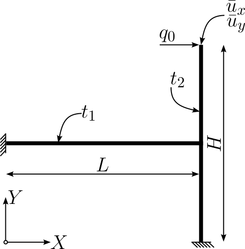
L = 50
H = 50
t_1 = 0.5
t_2 = 5
Force = 1e-2
2.1.2. Material Parameters#
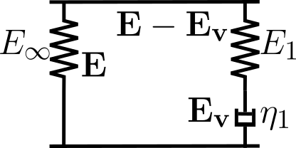
For the modeling of the viscoelastic behavior, we are using the generalized Maxwell Element as illustrated above. We assume an additive decomposition of the strains in terms of the Green strain tensor \(\mathbf{E}\).
The material is assumed incompressible. The viscoelastic model parameters are defined using a Prony Series with parameters \(g_1\) and \(\tau_1\) and the following relationships $\( E_1 = \frac{g_1}{1-g_1} E_{\infty},\\ \eta_1 = \tau_1 E_1. \)$
E = 3                           # Young's Modulus
nu = 0.5                        # Poisson Ratio
lam_material = E*nu/(1-nu**2)   # 1st Lame Constant with Plane Stress Consumptions
mu_inf = 0.5 / (1+nu) * E       # 2nd Lame Constant

g1 = 0.5                        # Prony Parameter
tau1 = 0.5                      # Prony Parameter

E1 = g1*E/(1-g1)                # Young's Modulus Viscoelastic Part
lam_1 = E1*0.5/(1-0.5**2)       # 1st Lame Constant with Plane Stress Consumptions Viscoelastic Part
mu_1 = g1*mu_inf/(1-g1)         # 2nd Lame Constant Viscoelastic PArt
eta1 = tau1*E1                  # Dashpoint Element
mat_horizontal = "mat_horizontal"
mat_vertical = "mat_vertical"
maxh = L/5
order = 3
2.2. Build Geometry by using OCC#
wire1 … horizontal part, wire2 … vertical part
pnt1 = Pnt(0,0,0)
pnt2 = Pnt(L,0, 0)
pnt3 = Pnt(L,H/2,0)
pnt4 = Pnt(L,-H/2,0)

wire1 = Wire([Segment(pnt1,pnt2)
             ])
wire2 = Wire([Segment(pnt2,pnt3),
             Segment(pnt4,pnt2)
             ])

face1 = wire1.Extrude((0,0,L))
face2 = wire2.Extrude((0,0,L))

# Name Edges for Boundary Conditions
face1.edges[0].name = "clamped_left"
face2.edges[1].name = "free"
face2.edges[4].name = "clamped_bottom"

# Mark Edges for refinement
face1.edges[0].hpref = 1
face2.edges[1].hpref = 1
face2.edges[4].hpref = 1
face2.edges[5].hpref = 1

for i in range (0,len(face1.vertices)):
    face1.vertices[i].hpref = 1

for i in range (0,len(face2.vertices)):
    face2.vertices[i].hpref = 1

# Name Faces in order to assign thickness
face1.faces.name = mat_horizontal
face2.faces[0].name = mat_vertical
face2.faces[1].name = mat_vertical

geometry1 = Glue([face1])
geometry2 = Glue([face2])
geometry = Glue([geometry1,geometry2])
Draw(geometry, settings={"camera": {"transformations": [{"type": "rotateY", "angle": 25},{"type": "rotateX", "angle": 25}]}})
BaseWebGuiScene
2.3. Mesh the above Geometry using RefineHP#
geo = OCCGeometry(geometry)
ngmesh = geo.GenerateMesh(maxh=maxh)
mesh = Mesh(ngmesh)
mesh.RefineHP(levels=2,factor=0.25)
mesh.Curve(order)

thickness_fun = mesh.BoundaryCF({mat_horizontal: t_1, mat_vertical: t_2})              # Assign Thickness to associated area
Draw(thickness_fun,mesh,'thickness', settings={"camera": {"transformations": [{"type": "rotateY", "angle": 25},{"type": "rotateX", "angle": 25}]}})
BaseWebGuiScene
2.4. FE Spaces#
Without going into the theory of the HHJ-shell method, we will refer to the various works by Schöberl, Neunteufel, Pechstein, et al.
For the analysis of the problem, we are using the following variables in the associated FE Space:
displacement
\(u \in \mathrm{H}^1(\Omega)^3\)
moment
\(\mathbf{m} \in \mathbf{H}(\mathrm{div}\ \mathrm{div})\)
hybridization vector
\(\boldsymbol{hyb} \in \mathbf{H}(\mathrm{div})\)
elastic membrane strain tensor
\(\mathbf{\varepsilon} \in \mathbf{H}(\mathrm{curl} \ \mathrm{curl})\)
viscoelastic membrane strain tensor
\(\mathbf{\varepsilon}_v \in \mathbf{H}(\mathrm{curl} \ \mathrm{curl})\)
elastic curvature tensor
\(\mathbf{\kappa} \in \mathbf{H}(\mathrm{curl} \ \mathrm{curl})\)
viscoelastic curvature tensor
\(\mathbf{\kappa}_v \in \mathbf{H}(\mathrm{curl} \ \mathrm{curl})\)
auxiliary variable (helps to reduce mebrane locking)
\(\mathbf{R} \in \mathbf{H}(\mathrm{curl} \ \mathrm{curl})\)
Green’s strain tensor is calculated by numerical integration over the thickness by \( \mathbf{E} = \mathbf{\varepsilon} + \zeta \mathbf{\kappa}\) and \( \mathbf{E}_v = \mathbf{\varepsilon}_v + \zeta \mathbf{\kappa}_v\).
Additionally, the boundary conditions are defined as dirichlet conditions in the displacements as well as dirichlet conditions in the hybridization space.
bbc_clamp = "clamped_left|clamped_bottom"
bbc_x = "clamped_left|clamped_bottom"
bbc_y = "clamped_left|clamped_bottom"
bbc_z = "clamped_left|clamped_bottom"

fes_mom = HDivDivSurface(mesh, order=order-1, discontinuous=True)
fes_u   = VectorH1(mesh, order=order, dirichletx_bbnd=bbc_x, dirichlety_bbnd=bbc_y, dirichletz_bbnd=bbc_z)
fes_hyb = HDivSurface(mesh, order=order-1, orderinner=0, dirichlet_bbnd=bbc_clamp)

fes_curlcurl = HCurlCurl(mesh, order=order, discontinuous=True)

fes  = fes_u*fes_hyb*fes_curlcurl*fes_curlcurl*fes_curlcurl*fes_mom*fes_curlcurl*fes_curlcurl
solution = GridFunction(fes, name="solution")           # Solution Function
u = solution.components[0]
solution_old = GridFunction(fes)                        # Solution Function of previous time step
print("Degrees of Freedom: ", sum(fes.FreeDofs(True)))
Degrees of Freedom: 4959
2.5. Special Functions and useful quantities#
Nsurf = specialcf.normal(mesh.dim)              # Surface normal N
t     = specialcf.tangential(mesh.dim)          # Tangential Vector
nel   = Cross(Nsurf, t)                         # In-plane edge normal

A  = Id(mesh.dim) - OuterProduct(Nsurf,Nsurf)   # First metric tensor

cfnphys = Normalize(Cof(A+Grad(u))*Nsurf)

gradN = specialcf.Weingarten(3)                 # Weingarten Tensor

fesVF = VectorFacetSurface(mesh, order=order)
averednv = GridFunction(fesVF)                  # averaged normal vector
averednv_start = GridFunction(fesVF)            # averaged initial normal vector

# Computation of averaged Normal Vector
n_ = fesVF.TrialFunction()
n_.Reshape((3,))

bfF = BilinearForm(fesVF, symmetric=True)
bfF += Variation( (0.5*n_*n_ - (cfnphys)*n_)*ds(element_boundary=True))

def ComputeAveredNV(averednv):
    rf = averednv.vec.CreateVector()
    bfF.Apply(averednv.vec, rf)
    bfF.AssembleLinearization(averednv.vec)
    invF = bfF.mat.Inverse(fesVF.FreeDofs())
    averednv.vec.data -= invF*rf

ComputeAveredNV(averednv)
ComputeAveredNV(averednv_start)

cfn  = Normalize(CoefficientFunction( averednv.components ))
cfnR = Normalize(CoefficientFunction( averednv_start.components ))  # nR

def SolveCondense(a, res, solver, w):
    if a.condense:
        res.data += a.harmonic_extension_trans * res
        w.data = solver * res
        w.data += a.harmonic_extension * w
        w.data += a.inner_solve * res
    else:
        w.data = solver * res

def SolveViscoTrapezoidalRule(a,b,X,X_0):
    rel_err = 1e-8
    abs_err = 1e-8
    max_it = 25

    freedofs = a.space.FreeDofs()
    freedofsb = b.space.FreeDofs()
    freedofs_c = a.space.FreeDofs(a.condense)

    res = X.vec.CreateVector()
    w = X_0.vec.CreateVector()

    res0 = X_0.vec.CreateVector()
    b.Apply(X_0.vec,res0)
    res0[~freedofsb] = 0.

    a.Apply(X.vec, res)
    res[~freedofs] = 0.
    init_norm_res = Norm(res)
    print(f'\t Initial Residuum = {init_norm_res}')
    j = 1
    while j <= max_it:
        a.AssembleLinearization(X.vec)
        inv = a.mat.Inverse(freedofs_c)

        SolveCondense(a, res, inv, w)
        X.vec.data -= w

        a.Apply(X.vec, res)
        res[~freedofs] = 0.
        res.data -= res0

        normres = Norm(res)

        if normres < rel_err * init_norm_res or normres < abs_err:
            print(f'\t Newton Step {j}: Residuum = {normres}')
            return j,0

        j+=1

    return j,Norm(res)
2.6. Test and Trial Functions#
u_, hyb_, eps_, R_, kappa_, mom_, eps_vi_, kappa_vi_ = fes.TrialFunction()[:8]
hyb_, eps_, R_, kappa_, mom_, eps_vi_, kappa_vi_ = hyb_.Trace(), eps_.Trace(), R_.Operator("dualbnd"), kappa_.Trace(), mom_.Trace(), eps_vi_.Trace(), kappa_vi_.Trace()

deps_vi, dkappa_vi = fes.TestFunction()[6:]
deps_vi, dkappa_vi = deps_vi.Trace(), dkappa_vi.Trace()

Fsurf_    = grad(u_).Trace() + A
Csurf_    = Fsurf_.trans*Fsurf_
epssurf_ = 0.5*(Csurf_ - A)

nphys   = Normalize(Cof(Fsurf_)*Nsurf)   # normal of deformed surface
tphys   = Normalize(Fsurf_*t)
nelphys = Cross(nphys,tphys)             # in-plane edge normal of deformed surface

Hn_ = CoefficientFunction( (u_.Operator("hesseboundary").trans*nphys), dims=(3,3) )       # Hessian of the displacement
pnaverage = Normalize( cfn - (tphys*cfn)*tphys )
2.7. BilinearForm#
Recalling the variational formulation in the form $\( \delta\Psi+\frac{\partial\phi}{\partial\dot{\mathbf{E}_v}}\colon\delta\mathbf{E}_v+\delta W_{\text{ext}}=0, \)\( and using the dissipation function as \)\( \phi = \frac{2}{3}\frac{1}{2}\eta_1{\left|\dot{\mathbf{E}_v}\right|}^2, \)\( the second term can be rewritten as \)\( \frac{\partial\phi}{\partial\dot{\mathbf{E}_v}}\colon\delta\mathbf{E}_v=\frac{2}{3}\eta_1\dot{\mathbf{E}_v}\colon\delta\mathbf{E}_v. \)\( Starting at \)t_0\(, where the solution is known, the next time step \)t_0+\Delta t\( can be determined by solving \)\( \int_{t_0}^{t_0+\Delta t} \left(\frac{2}{3}\eta_1\dot{\mathbf{E}_v}\colon\delta\mathbf{E}_v d\tau\right)=\int_{t_0}^{t_0+\Delta t} \left(-\delta\Psi-\delta W_{\text{ext}}\right)d\tau. \)\( First of all, the result of the left hand side of the above equation is to be determined. \)\( \frac{2}{3}\eta_1 \int_{t_0}^{t_0+\Delta t} \left(\dot{\mathbf{E}_v}\colon\delta\mathbf{E}_v d\tau\right)=\frac{2}{3}\eta_1 \left({\mathbf{E}_v}\left(t_0+\Delta t\right)-{\mathbf{E}_v}\left(t_0\right)\right)\colon\delta\mathbf{E}_v \)\( This result leads to \)\( \frac{2}{3}\eta_1 \left({\mathbf{E}_v}\left(t_0+\Delta t\right)-{\mathbf{E}_v}\left(t_0\right)\right)\colon\delta\mathbf{E}_v=\underbrace{\int_{t_0}^{t_0+\Delta t} \left(-\delta\Psi-\delta W_{\text{ext}}\right)d\tau}_{\text{Time Integration Method}}, \)$ where the time integration method has to be chosen.
Using the trapezoidal rule, the right hand side from above gives $\( -\Delta t\left(\frac{1}{2}\left(\delta\Psi \big|_{t_0+\Delta t}+\delta\Psi \big|_{t_0}\right) + \frac{1}{2}\left(\delta W_{\text{ext}} \big|_{t_0+\Delta t}+ \delta W_{\text{ext}} \big|_{t_0}\right)\right). \)\( For the fininte element analysis, the equation is used in the following form with two bilinear forms \)a\( and \)b\( \)\( \underbrace{\frac{2}{3}\eta_1 \left({\mathbf{E}_v}\left(t_0+\Delta t\right)-{\mathbf{E}_v}\left(t_0\right)\right)\colon\delta\mathbf{E}_v+\frac{\Delta t}{2}\left(\delta\Psi \big|_{t_0+\Delta t}+\delta W_{\text{ext}} \big|_{t_0+\Delta t}\right)}_{=:a} = -\underbrace{\frac{\Delta t}{2}\left(\delta\Psi \big|_{t_0}+\delta W_{\text{ext}} \big|_{t_0}\right)}_{=:b}. \)$
par = Parameter(0)      # Load Parameter used for load stepping
par0 = Parameter(0)     # Previous Load Parameter
DeltaT = Parameter(0)   # Time Step

gausspoints  = [(-np.sqrt(3/7+2/7*np.sqrt(6/5)), (18-np.sqrt(30))/36 ),
               (-np.sqrt(3/7-2/7*np.sqrt(6/5)), (18+np.sqrt(30))/36 ),
               (np.sqrt(3/7-2/7*np.sqrt(6/5)), (18+np.sqrt(30))/36 ),
               (np.sqrt(3/7+2/7*np.sqrt(6/5)), (18-np.sqrt(30))/36 )  ]     # Used for numerical integration in thickness directions

def BuildBF(rhs = False):
    fac = -1 if rhs else 1
    bf = BilinearForm(fes, symmetric=True, condense=True, printelmat=False)

    for (zi, wi) in gausspoints:                # thickness Integration
        zeta = thickness_fun/2*zi
        weightdet = wi*thickness_fun/2

        E_       = eps_   + zeta*kappa_
        E_vi_    = eps_vi_ + zeta*kappa_vi_
        delE_    = E_-E_vi_

        FB =  A
        III_Lambda = (Cof(FB)*Nsurf)*Nsurf

        SVK = mu_inf*InnerProduct(E_,E_)+0.5*lam_material*Trace(E_)**2
        SVK_VI = mu_1*InnerProduct(delE_,delE_)+0.5*lam_1*Trace(delE_)**2

        bf += Variation(fac*(SVK)*weightdet*III_Lambda*ds).Compile()
        bf += Variation(fac*(SVK_VI)*weightdet*III_Lambda*ds).Compile()

        if not rhs:
            Eps_vi_last = solution_old.components[6]
            kappa_vi_last = solution_old.components[7]
            E_vi_last = Eps_vi_last+zeta*kappa_vi_last

            Eps_vi_dot = (E_vi_-E_vi_last)

            bf += SymbolicBFI(2/DeltaT*2/3*eta1*(InnerProduct(Eps_vi_dot,deps_vi+zeta*dkappa_vi)+
                                                InnerProduct(Eps_vi_dot,A)*
                                                InnerProduct(deps_vi+zeta*dkappa_vi,A))*weightdet*III_Lambda,BND)

    bf += Variation( fac*(-InnerProduct(mom_, kappa_ + Hn_ + (1-nphys*Nsurf)*gradN))*ds ).Compile()

    bf += Variation( fac*InnerProduct(eps_-epssurf_, R_)*ds(element_vb=BND ) )
    bf += Variation( fac*InnerProduct(eps_-epssurf_, R_)*ds(element_vb=VOL ) )
    bf += Variation( fac*(acos(nel*cfnR)-acos(nelphys*pnaverage)-hyb_*nel)*(mom_*nel)*nel*ds(element_boundary=True ) ).Compile()

    if rhs:
        bf += Variation(-fac*par0*Force*t_2*u_[0]*ds(definedon=mesh.BBoundaries("free"))).Compile()
    else:
        bf += Variation(-fac*par*Force*t_2*u_[0]*ds(definedon=mesh.BBoundaries("free"))).Compile()
    return bf

bfa = BuildBF(rhs=False)
bfb = BuildBF(rhs=True)
solution.vec[:] = 0

t1 = 5                      # Time period
nsteps_load = 5             # number of load steps
nsteps_relaxation = 25      # number of relaxation steps

time_vec = np.append(np.linspace(0,1e-5,nsteps_load,endpoint=False),np.linspace(1e-5,t1,nsteps_relaxation))
load_vec = np.append(np.linspace(0,1,nsteps_load,endpoint=False),np.linspace(1,1,nsteps_relaxation))
disp_x = []
time_sol = []
disp_y = []
disp_x += [0]
time_sol += [0]
disp_y += [0]
solution.vec[:] = 0
for i in range(len(time_vec))[1:]:
    print(f'{np.round(time_vec[i],3)} seconds, total time: {t1} seconds')
    solution_old.vec.data = solution.vec
    par.Set(load_vec[i])
    par0.Set(load_vec[i-1])
    DeltaT.Set(time_vec[i]-time_vec[i-1])

    with TaskManager():
        idx, res = SolveViscoTrapezoidalRule(bfa,bfb,solution,solution_old)
        if res != 0:
            print(f'\t Newton did not converge! Residuum = {res}')
            break

    rhs = solution.vec.CreateVector()
    bfa.Apply(solution.vec, rhs)

    int0 = Integrate(1, mesh, definedon=mesh.BBoundaries("free"))
    u_sol = Integrate(solution.components[0], mesh, definedon=mesh.BBoundaries("free"))
    u_x = 1/int0 * u_sol[0]
    u_y = 1/int0 * u_sol[1]

    time_sol += [time_vec[i]]
    disp_x += [u_x]
    disp_y += [u_y]
    Redraw()
0.0 seconds, total time: 5 seconds
Initial Residuum = 0.2008256611605077
Newton Step 4: Residuum = 1.2285174385098356e-10
0.0 seconds, total time: 5 seconds
Initial Residuum = 8.883197530540022
Newton Step 3: Residuum = 3.765627610898331e-08
0.0 seconds, total time: 5 seconds
Initial Residuum = 17.593227129504065
Newton Step 3: Residuum = 3.127794508803122e-08
0.0 seconds, total time: 5 seconds
Initial Residuum = 26.02092517098512
Newton Step 3: Residuum = 2.673677708289189e-08
0.0 seconds, total time: 5 seconds
Initial Residuum = 34.08092517135217
Newton Step 3: Residuum = 2.0666167613701468e-08
0.208 seconds, total time: 5 seconds
Initial Residuum = 41.720558736007156
Newton Step 4: Residuum = 9.449518014068606e-11
0.417 seconds, total time: 5 seconds
Initial Residuum = 33.01881142283049
Newton Step 4: Residuum = 1.007963093888907e-10
0.625 seconds, total time: 5 seconds
Initial Residuum = 26.068960385703374
Newton Step 4: Residuum = 1.1304690971218879e-10
0.833 seconds, total time: 5 seconds
Initial Residuum = 20.54762381765454
Newton Step 4: Residuum = 1.0230827672668795e-10
1.042 seconds, total time: 5 seconds
Initial Residuum = 16.17710343454419
Newton Step 4: Residuum = 8.197431988687177e-11
1.25 seconds, total time: 5 seconds
Initial Residuum = 12.726203351615208
Newton Step 4: Residuum = 8.975034064358683e-11
1.458 seconds, total time: 5 seconds
Initial Residuum = 10.006152411198421
Newton Step 4: Residuum = 1.1250751253102791e-10
1.667 seconds, total time: 5 seconds
Initial Residuum = 7.864747779400751
Newton Step 3: Residuum = 4.749642662788863e-08
1.875 seconds, total time: 5 seconds
Initial Residuum = 6.180292236371997
Newton Step 3: Residuum = 1.7860108615557005e-08
2.083 seconds, total time: 5 seconds
Initial Residuum = 4.856029337759428
Newton Step 3: Residuum = 6.7279522397700626e-09
2.292 seconds, total time: 5 seconds
Initial Residuum = 3.815331136416084
Newton Step 3: Residuum = 2.5388517025730564e-09
2.5 seconds, total time: 5 seconds
Initial Residuum = 2.9976750890375747
Newton Step 3: Residuum = 9.620465457874135e-10
2.708 seconds, total time: 5 seconds
Initial Residuum = 2.3553498204292627
Newton Step 3: Residuum = 3.7754883683724784e-10
2.917 seconds, total time: 5 seconds
Initial Residuum = 1.8507934465933122
Newton Step 3: Residuum = 1.6621048093997903e-10
3.125 seconds, total time: 5 seconds
Initial Residuum = 1.454462165311802
Newton Step 3: Residuum = 1.1604141660525844e-10
3.333 seconds, total time: 5 seconds
Initial Residuum = 1.1431337716021102
Newton Step 3: Residuum = 1.0759827254835382e-10
3.542 seconds, total time: 5 seconds
Initial Residuum = 0.8985631285366471
Newton Step 3: Residuum = 9.254079555197442e-11
3.75 seconds, total time: 5 seconds
Initial Residuum = 0.7064196700278188
Newton Step 3: Residuum = 1.0728268694859673e-10
3.958 seconds, total time: 5 seconds
Initial Residuum = 0.5554496220371844
Newton Step 3: Residuum = 1.0808240993526598e-10
4.167 seconds, total time: 5 seconds
Initial Residuum = 0.43681631882300054
Newton Step 3: Residuum = 8.441149599607483e-11
4.375 seconds, total time: 5 seconds
Initial Residuum = 0.3435813902388205
Newton Step 3: Residuum = 9.682126354759739e-11
4.583 seconds, total time: 5 seconds
Initial Residuum = 0.27029695350074995
Newton Step 3: Residuum = 1.1469897375380307e-10
4.792 seconds, total time: 5 seconds
Initial Residuum = 0.21268531522903647
Newton Step 3: Residuum = 9.324184292698437e-11
5.0 seconds, total time: 5 seconds
Initial Residuum = 0.16738740505581712
Newton Step 3: Residuum = 1.1271915603430923e-10
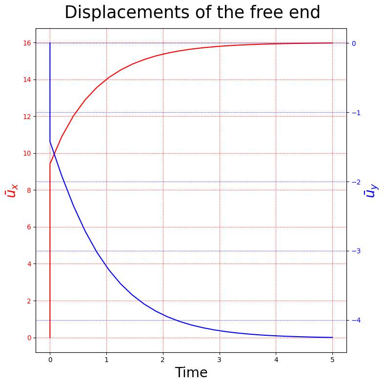
fig, ax = plt.subplots(1,1, figsize=(8,8))
fig.suptitle("Displacements of the free end", size=25)
ax.plot(time_sol, disp_x, color = 'red')
ax.set_xlabel(r'Time', size=20)
ax.set_ylabel(r'$\bar{u}_x$',color = 'red', size=20)
ax.grid(color='red', linestyle='dotted')
ax.tick_params(axis='y', labelcolor='red')

ax2 = ax.twinx()
ax2.plot(time_sol,disp_y,color='blue',label='Displacement y')
ax2.set_ylabel(r'$\bar{u}_y$',color = 'blue', size=20)
ax2.tick_params(axis='y', labelcolor='blue')
ax2.grid(color='blue', linestyle="dotted")
fig.tight_layout()
print('Norm(displacement):')
Draw(solution.components[0][0], mesh, "displacement", deformation=solution.components[0], settings={"camera": {"transformations": [{"type": "rotateY", "angle": 25},{"type": "rotateX", "angle": 25}]}})
print('Norm(eps_v):')
Draw(Norm(solution.components[6]), mesh, "viscoelastic strains", deformation=solution.components[0], settings={"camera": {"transformations": [{"type": "rotateY", "angle": 25},{"type": "rotateX", "angle": 25}]}})
print('Norm(kappa_v):')
Draw(Norm(solution.components[4]), mesh, "viscoelastic curvature", deformation=solution.components[0], autoscale=False, min=0, max=0.05,settings={"camera": {"transformations": [{"type": "rotateY", "angle": 25},{"type": "rotateX", "angle": 25}]}})
Norm(displacement):
Norm(eps_v):
Norm(kappa_v):
BaseWebGuiScene