3. Space charge problem applied to HVDC power transmission

Madeline Chauvier

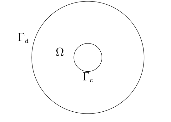
We want to find a couple of solution \((\rho,\varphi)\) on a domain \(\Omega\) to the system :

\[\begin{align*} \Delta \varphi = -\rho \quad &\text{in } \Omega\\ \nabla \cdot (\rho \nabla \varphi) = 0 \quad &\text{in } \Omega \\ \varphi = 1, \quad &\text{on } \Gamma_c, \\ \varphi = 0, \quad &\text{on } \Gamma_d, \\ \nabla \varphi \cdot n = A,\quad &\text{on } \Gamma_c. \end{align*}\]

where \(\varphi\) is the potential of the electric field and \(\rho\) is the positive charge density. \(A\) is a constant and \(\Gamma_c\) is the boundary of the conductor (interior boundary) and \(\Gamma_d\) is the air or the ground (exterior boundary).

from netgen.geom2d import CSG2d, Circle, Rectangle
from ngsolve import *
import ngsolve
import numpy as np
import scipy
from ngsolve.webgui import Draw
from ngsolve import Mesh, VOL

3.1. Generate mesh on the domain

geo = CSG2d()
cercle_ext = Circle(center = (0,0), radius = 1.0, bc = "label_ext")
circle_int = Circle(center = (0,0), radius = 0.5, bc = "label_int")
domain = cercle_ext-circle_int
geo.Add(domain)
m = geo.GenerateMesh(maxh = 0.1)
mesh = Mesh(m)
Draw(mesh)

BaseWebGuiScene

    
def discret_to_grid(tab : np.ndarray, flag : bool) -> GridFunction:
    """
    Transform an array (tab) to a GridFunction

    Parameters
    ----------
    tab : np.ndarray
        discret function on H1

    Out
    -------
    GridFunction : tab transformed in GridFunction 

    Error
    -------
    IndexError : if the size of the array doesn't correspond to the mesh
    """
    if flag == True:
        fes = H1(mesh, order = 1)
    else:
        fes = L2(mesh, order = 1)
    gf = GridFunction(fes)
    if not gf.vec.size == len(tab):
        raise IndexError
    gf.vec[:] = tab
    return gf 
    

3.2. Solving Process

Let \(\rho\) be fixed and one solve the system for \(\varphi\). We divide the system into two systems. The first one is :

\[\begin{align*} \Delta \varphi = -\rho \quad &\text{in } \Omega\\ \varphi = 0, \quad &\text{on } \Gamma_d, \\ \nabla \varphi \cdot n = A,\quad &\text{on } \Gamma_c. \end{align*}\]

A = 1.5      

def solve_phi1(ρ : GridFunction) -> GridFunction:
    """
    Solve the equation Δφ = -ρ in φ where ρ is fixed with the mixte condition on the boundary ie : ∇φ n=-A on the interior boundary ,φ=0 on the exterior boundary

    Parameter:
    ------------
    ρ : GridFunction
        ρ discret on the mesh
    
    Out:
    --------
    GridFunction : φ discret on the mesh
    """
    fes = H1(mesh, order = 1, dirichlet = "label_ext")
    uD = CF(0)
    uN = mesh.BoundaryCF({'label_int':A}, default = 0)
    sol = GridFunction(fes)
    u,v = fes.TnT()
    a = BilinearForm(grad(u)*grad(v)*dx).Assemble()
    f = LinearForm(ρ*v*dx + uN*v*ds).Assemble()
    sol.Set(uD,BND)
    c= Preconditioner(a, "local")
    c.Update()
    solvers.BVP(bf = a, lf = f, gf = sol, pre = c, print = False)
    return sol

Then, we solve :

\[\begin{align*} \nabla \cdot (\rho \nabla \varphi) = 0 \quad &\text{in } \Omega \\ \varphi = 1, \quad &\text{on } \Gamma_c, \\ \varphi = 0, \quad &\text{on } \Gamma_d \end{align*}\]

def solve_phi2(ρ: GridFunction) ->  GridFunction:
    """
    Solve the equation -∇ ∙ ((ρ+1) ∇φ) =ρ  with the Dirichlet conditions on the boundaries, ie : φ=0 on the exterior circle and φ = 1 on the interior circle

    Paramètres :
    -----------
    ρ : GridFunction   
        ρ discret on the mesh
        
    Sortie:
    --------
    sol : Gridfunction
        function solution on the mesh
    """
   
    fes = H1(mesh, order = 1, dirichlet = "label_ext|label_int")
    g = mesh.BoundaryCF({"label_ext":0 , "label_int":1}, default = 0)
    u,v = fes.TnT()
    a = BilinearForm((ρ+1)*grad(u)*grad(v)*dx).Assemble()
    f = LinearForm(ρ*v*dx).Assemble() 
    sol = GridFunction(fes)
    sol.Set(g,BND)
    c= Preconditioner(a, "local")
    c.Update()
    solvers.BVP(bf = a, lf = f, gf = sol, pre = c, print = False)
    return sol

3.3. Minimisation algorithm

For solving the whole system, we will minimize the function \(J(\rho) = 1/2 |\nabla \varphi_1-\nabla \varphi_2|_2^2\) where \(\varphi_1\) (resp. \(\varphi_2\)) is the solution for the first (resp. second) system. So, we need to calculate the gradient of the function \(J\). So we need to solve the following equation, for \(u = \nabla J(\rho)\) :

\[\begin{align*} \int_\Omega u z + \nabla u \nabla z dx = \int_\Omega \nabla(\varphi_1-\varphi_2) \nabla(\partial_\rho \varphi_1 [z]- \partial_\rho \varphi_2[z]) dx. \end{align*}\]

Here, we had a problem because in the right member of this equality, we can see that the test function \(z\) is not explicit (it’s hidden in the differential). For solving this problem, we solve an intermediate system for \(\Psi\):

\[\begin{align*} \nabla \cdot \Bigl((\rho(x) +1) \nabla \Psi(x)\Bigr) = \Delta (\varphi_1(x) -\varphi_2(x)), & \hspace*{1ex} \text{ pour } x \in \Omega, \\ \Psi(x) = 0, & \hspace*{1ex} \text{ pour } x \in \partial \Omega. \end{align*}\]

def solve_psi(ϕ1 : GridFunction, ϕ2 : GridFunction, ρ : GridFunction) -> GridFunction:
    """
    Solve the equation -∇ ∙ ((ρ+1) ∇ψ) = Δ(ϕ1-ϕ2) with Dirichlet boundary ie ψ = 0 
    Parameter:
    ----------
    ϕ1 : Gridfunction
        function solution obtained by solve_phi1
    ϕ2 : GridFunction
        function solution obtained by solve_phi2
    ρ : GridFunction
        ρ discret on the mesh
    
    Out:
    --------
    GridFunction : function solution on the mesh
    """
    fes = H1(mesh, order = 1, dirichlet = "label_ext|label_int")
    g = mesh.BoundaryCF({"label_ext":0, "label_int":0}, default = 0)
    u,v = fes.TnT()
    a = BilinearForm((ρ+1)*grad(u)*grad(v)*dx).Assemble()
    fes_H0 = H1(mesh, order = 1, dirichlet = "label_ext")
    soustract = GridFunction(fes_H0)
    soustract.Set(ϕ1-ϕ2)
    f = LinearForm(grad(soustract)*grad(v)*dx).Assemble() 
    sol = GridFunction(fes)
    sol.Set(g,BND)
    c= Preconditioner(a, "local")
    c.Update() 
    solvers.BVP(bf = a, lf = f, gf = sol, pre = c, print = False)
    return sol


def grad_J(ρ : np.ndarray) -> np.ndarray:
    """
    Calculate the gradient of the function to minimize in H1

    Parameter
    -----------
    ρ : np.ndarray
        ρ as an array
    
    Sortie
    -------
    np.ndarray : gradient of J 
    """
    ρ_grid = discret_to_grid(ρ, True)
    ϕ1 = solve_phi1(ρ_grid)
    ϕ2 = solve_phi2(ρ_grid)
    psi = solve_psi(ϕ1, ϕ2, ρ_grid)
    fes = H1(mesh, order=1)
    u,v = fes.TnT()
    sol = GridFunction(fes)
    a = BilinearForm(grad(u)*grad(v)*dx + u*v*dx).Assemble()
    f = LinearForm((ϕ1-ϕ2-psi + grad(ϕ2)*grad(psi))*v*dx)
    c = Preconditioner(a, "local")
    c.Update()
    solvers.BVP(bf = a, lf = f, gf = sol, pre = c, print = False)
    grad_J_array = np.array(sol.vec)
    return grad_J_array

3.4. Minimization

We define the function \(J\) and we minimize it.

def inner_H1_0(u : GridFunction,v : GridFunction) -> float:
        """
        Calculate the scalar product H¹₀

        Parameter:
        ----------
        u, v : Gridfunction

        Out
        -------
        float : scalar product H¹₀ of u and v
        """
        fes = H1(mesh, order = 1, dirichlet = "label_ext|label_int")
        u_H1_0,v_H1_0 = fes.TnT()
        a = BilinearForm(grad(u_H1_0)*grad(v_H1_0)*dx).Assemble()
        return InnerProduct(u.vec,a.mat*v.vec)

def norme_H1_0_carre(u : GridFunction) -> float:
    """
    Calculate the norm H¹₀ to the square

    Parameter
    ----------
    u : Grifunction

    Out
    --------
    float : norm H¹₀ to the square of u
    """
    return inner_H1_0(u,u)


def J(ρ : np.ndarray) -> float:
    """
    Calculate the function to minimize, J

    Parameter
    ---------
    ρ : np.ndarray
        ρ discret as an array
    """
    ρ_grid = discret_to_grid(ρ,True)
    ϕ1 = solve_phi1(ρ_grid)
    ϕ2 = solve_phi2(ρ_grid)
    fes = H1(mesh, order = 1, dirichlet = "label_ext")
    soustract = GridFunction(fes)
    soustract.Set(ϕ1-ϕ2)
    return 1/2 * norme_H1_0_carre(soustract)

def minimize(ρ : np.ndarray):
    """
    Minimize function
    
    """
    min = scipy.optimize.minimize(J, ρ,
                                method = "L-BFGS-B", jac = grad_J, tol = 1e-9, options = {'ftol' : 1e-9, 'gtol' : 1e-9})
    return min

import matplotlib.pyplot as plt
from ngsolve import *
import ngsolve
import math
import matplotlib.tri as mtri


def rho(x,λ,r_0):
    if λ >=-1:
        return λ/((f(λ,r_0,1)-f(λ,r_0,r_0))*sqrt(λ*x**2+1))
    elif λ <= -1/r_0**2:
        return  -λ/((f(λ,r_0,1)-f(λ,r_0,r_0))*sqrt(-λ*x**2-1))

def f(λ,r_0,x):
    if λ >=-1:
        return sqrt(1+λ*x**2)- log(sqrt(1+λ*x**2)+1)+log(x)
    if λ <= -1/r_0**2:
        return sqrt(-λ*x**2-1)-atan(sqrt(-λ*x**2-1))

def A_lambda(λ):
    return math.sqrt(abs(λ+1/r_0**2))/ (f(λ,r_0,1)-f(λ,r_0,r_0))


def ϕ(λ,r_0,x):
    return (f(λ,r_0,1)-f(λ,r_0,x))/(f(λ,r_0,1)-f(λ,r_0,r_0))

r_0 = 0.5
λ = -10

fes = H1(mesh, order = 1)



ρ_grid = GridFunction(fes)
ρ_grid.Set(x+y +4) 
ρ_array = np.array(ρ_grid.vec)
ρ_init = ρ_array


res_H1 = minimize(ρ_array)
print("H1",res_H1.nit, res_H1.success, res_H1.status, res_H1.message)
ρ_sol_grid_H1 = discret_to_grid(res_H1.x, True)
phi1_H1 = solve_phi1(ρ_sol_grid_H1)
phi2_H1 = solve_phi2(ρ_sol_grid_H1)


triangles = []

for el in mesh.Elements(VOL): 
    v = el.vertices
    triangles.append([v[0].nr, v[1].nr, v[2].nr])


fig = plt.figure()
ax = fig.add_subplot(2,2,1,projection ='3d')

X = np.array([v.point[0] for v in mesh.vertices])
Y = np.array([v.point[1] for v in mesh.vertices])

triang = mtri.Triangulation(X,Y,triangles = triangles)
ax.plot_trisurf(triang, np.array(phi1_H1.vec), label = "phi1", cmap = plt.cm.Spectral)
ax.legend()


ax = fig.add_subplot(2,2,2, projection = '3d')

ax.plot_trisurf(triang, np.array(phi2_H1.vec), label = "phi2", cmap = plt.cm.Spectral)
ax.legend()

ax = fig.add_subplot(2,2,3, projection = '3d')

ax.plot_trisurf(triang, np.array(res_H1.x), label = "rho_num", cmap = plt.cm.Spectral)
ax.legend()


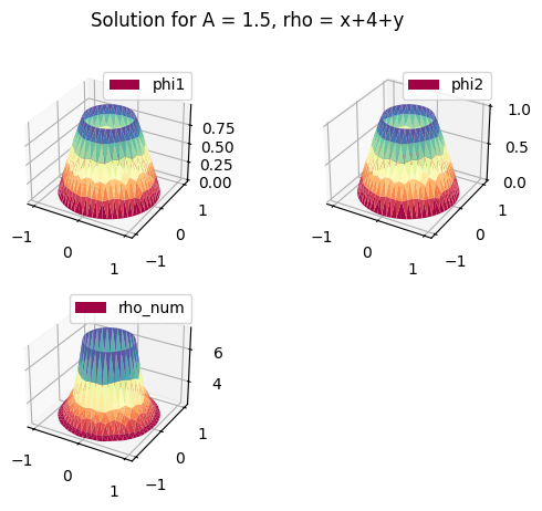
fig.suptitle("Solution for A = 1.5, rho = x+4+y")

plt.show()

no more timer available (FESpace), reusing last one

H1 105 True 0 CONVERGENCE: REL_REDUCTION_OF_F_<=_FACTR*EPSMCH

from ngsolve.webgui import Draw


Draw(ρ_sol_grid_H1)

BaseWebGuiScene

Draw(phi1_H1)

BaseWebGuiScene

Draw(phi2_H1)

BaseWebGuiScene